🏠 Building Model#
The building-scale model characterizes the optimal design and operation of a Building Energy System (BES): a set of energy conversion and storage technologies that interface local resources and imported energy supplies with the end-users’ energy services.
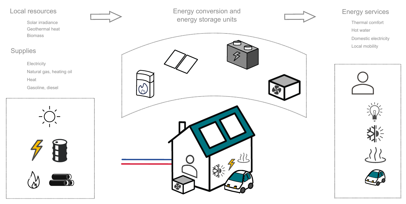
Building energy hub: conversion and storage units interface local resources and imported energy with end-users’ services.#
A Mixed-Integer Linear Programming (MILP) formulation simultaneously optimizes the selection, sizing and operation of all technologies. Multi-objective optimization via \(\epsilon\)-constraints enables trade-offs between economic and environmental criteria.
MILP formulation#
Problem structure#
A building is characterized by hourly energy service demand profiles. The BES satisfies these demands through equipment that can either harvest local resources (solar irradiance, geothermal heat) or purchase energy from utilities (electricity, natural gas, heating oil, etc.), depending on available grid connections.
Note
The model is defined on an hourly basis for a full year but a data reduction method (see Data reduction and typical periods) reduces the problem to typical periods \(p \in \mathbb{P}\), each with \(t \in \mathbb{T}\) timesteps (usually 24 h per representative day).
Note
Although defined for a single building, all equations carry the subscript \(b\) to prepare for the district-scale extension in 🏙️ District Model.
Constraints#
Unit selection and sizing#
The decision to install technology \(u\) in building \(b\) is captured by the binary variable \(\boldsymbol{y}_{b,u}\); the continuous variable \(\boldsymbol{f}_{b,u}\) is its installed capacity. Capacity bounds \(F_u^{\min}\) and \(F_u^{\max}\) also define the validity range of the linearized cost function.
Energy balance#
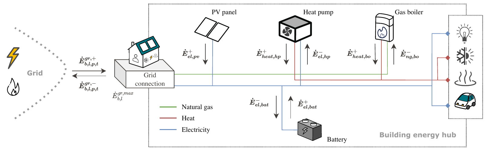
Energy balance in the building energy hub through grid exchanges and unit conversions.#
At every timestep the energy withdrawn from the grid plus the energy delivered by units must equal the energy injected back plus the energy consumed by units and the direct end-use demand (EUD):
Note
Heat layer vs. heat cascade. The heat layer represents energy purchased from a district heating network. The heat cascade is an internal building model of hot/cold streams discretized into temperature intervals; it enforces the second law of thermodynamics and tracks nominal supply/return temperatures of the heat distribution system.
Thermal load calculation#
Unlike DHW and electricity demands (parameterized timeseries), the space heating/cooling load \(\dot{\boldsymbol{Q}}_{b,p,t}\) is a decision variable, capturing control strategy and thermal mass effects:
Parameter |
Description |
|---|---|
\(\dot{Q}_{b,p,t}^{\text{gain}}\) |
Internal + solar heat gains |
\(A^{\text{era}}_b\) |
Energy reference area (ERA) |
\(U_b\) |
Overall heat transfer coefficient (conduction + ventilation) |
\(C_b\) |
Thermal heat capacity |
\(\boldsymbol{T}^{\text{int}}_{b,p,t}\) |
Indoor temperature (decision variable) |
\(T^{\text{ext}}_{p,t}\) |
Outdoor temperature (parameter) |
The building’s thermal mass acts as free, implicit thermal storage — surplus renewable electricity can be used to pre-heat or pre-cool the building.
Internal temperature setpoint#
Thermal comfort is enforced via hard bounds (absolute limits always enforced) and soft bounds (violations are penalized):
Deviations from the time-dependent soft comfort range \([T^{\min}_{b,p,t},\, T^{\max}_{b,p,t}]\) incur a penalty:
The coefficient \(c^{\text{pen}}_b\) [CHF/°C/h] quantifies the end user’s willingness to pay for thermal comfort. The total annual penalty for building \(b\) is added to the objective:
Grid usage constraint#
Peak power exchange with the grid is bounded per energy layer:
The grid usage coefficient \(\boldsymbol{GU}_{b}^{\pm}\) normalizes peak exchange relative to peak uncontrollable domestic demand — useful as an \(\epsilon\)-constraint to limit grid strain from electrification:
Objective functions#
Operating expenditures (OPEX)#
Annual costs from energy imports and exports across all layers, weighted to represent a full year:
An optional grid connection cost (fixed \(k_l^1\) + demand-charge \(k_l^2\)) can be added:
Capital expenditures (CAPEX)#
Investment and replacement costs are annualized using the capital recovery factor:
Here \(n\) is the project horizon, \(i\) the interest rate, \(n_u\) the technical lifetime of unit \(u\), and \(r \in \mathbb{R}\) indexes replacement events within the horizon. Multiple pairs \((c_u^1, c_u^2)\) can be defined for the same unit type, each valid over a different capacity interval \([F_u^{\min}, F_u^{\max}]\), enabling piecewise-linear cost approximations.
Total expenditures (TOTEX)#
Global warming potential (GWP)#
Environmental impact is expressed in CO₂ equivalents, split into operational and construction components:
Carbon content parameters \(cc^+_{l,p,t}\) are time-varying for electricity (reflecting renewable penetration), and constant for fossil carriers. Carbon content of technologies (\(cc_u^1\), \(cc_u^2\)) is derived from the ecoinvent life-cycle database.
Multi-objective optimization via \(\epsilon\)-constraints#
The problem is solved as a multi-objective optimization (MOO) using the \(\epsilon\)-constraint method. One objective (e.g., OPEX) is minimized while the other (e.g., CAPEX or GWP) is bounded by a parameter \(\epsilon\). Repeating this for increasing \(\epsilon\) values traces the Pareto frontier and reveals the trade-off between economic and environmental performance.
Data reduction and typical periods#
An hourly annual model has 8 760 timesteps — too many for tractable district-scale MILP. A K-Medoids clustering aggregates the year into \(|\mathbb{P}|\) typical days (usually 10–15), each assigned a weight \(d_p\) proportional to its number of occurrences. Clustering features include temperature, irradiance, weekday type, and optionally carbon intensity of the grid or ICT demand profiles.
Weights \(d_p\) (days/year) and \(d_t\) (hours/timestep) are used throughout to recover annual totals from the reduced set of operating hours.
End-use demand profiles#
Electricity demand#
When measured data are unavailable, electricity demand is synthesized from the SIA 2024 norm per room type \(r\) and building use:
Domestic hot water (DHW)#
DHW demand per building follows the same norm-based approach but with a specific thermal demand term \(\dot{q}^{\text{dhw}}_{r,p,t}\) (incorporating water heat capacity and the 10 °C → 60 °C temperature rise):
Note
Unlike electricity — which must be satisfied at every timestep — DHW production timing is flexible: the model couples any DHW-producing unit with a hot water storage tank, requiring only the daily volume and temperature to be met. This creates an opportunity to maximize on-site renewable self-consumption.
Heating and cooling demand#
Space heating and cooling demands are the positive and negative parts of the thermal load \(\dot{\boldsymbol{Q}}_{b,p,t}\) from (4). Key parameters influencing this demand are:
Occupancy profiles (effect on \(\dot{Q}^{\text{gain}}\))
Envelope quality \(U_b\)
Soft comfort bounds \(T^{\min}_{b,p,t}\), \(T^{\max}_{b,p,t}\) (time-dependent, e.g., relaxed at night)
Penalty coefficient \(c^{\text{pen}}_b\) [CHF/°C/h]
Free-cooling strategies (opening windows) can be modeled by allowing direct heat rejection when \(T^{\text{ext}}_{p,t} \le T^{\min}_{b,p,t}\).
Mobility demand#
Private car mobility is described by a plug-out factor \(\alpha_{p,t} \in [0,1]\): the fraction of time during \((p,t)\) when the vehicle is away from the building. Separate weekday and weekend templates are derived from national transport statistics:
The daily driving energy per vehicle is:
where \(d^{\text{day}}\) [km/person/day], \(n_{\text{pers/EV}}\) [persons/car], and \(\varepsilon_{\text{EV}}\) [kWh/km] connect population mobility needs to per-vehicle energy.
ICT demand#
Buildings can optionally include an integrated data-center module that introduces a dedicated ICT energy layer, linking server load to electricity consumption and waste heat recovery. See the reference thesis (Chapter 2) for the full formulation.
Energy layers#
The table below summarizes the energy layers implemented for buildings with default cost and carbon content assumptions. These values are context-dependent and must be calibrated for each case study.
Layer |
Supply cost \(c^+\) [CHF/kWh] |
Feed-in price \(c^-\) [CHF/kWh] |
Supply GWP \(cc^+\) [gCO₂eq/kWh] |
Feed-in GWP \(cc^-\) |
|---|---|---|---|---|
Electricity |
0.330 |
0.170 |
130 |
−130 |
Natural gas |
0.140 |
— |
230 |
— |
Heating oil |
0.120 |
— |
280 |
— |
Heat (DHN) |
0.150 |
0.050 |
190 |
— |
Wood pellets |
0.110 |
— |
90 |
— |
Hydrogen |
0.450 |
0.150 |
320 |
— |
Biomethane |
0.200 |
— |
180 |
— |
Gasoline |
0.190 |
— |
385 |
— |
CO₂ |
— |
— |
— |
— |
Data |
— |
— |
— |
— |
Note
Negative feed-in GWP for electricity reflects the assumption that exported electricity displaces marginal grid electricity and thus reduces grid carbon content. The embodied impact of PV panels is already accounted for in \(\boldsymbol{GWP}^{\text{constr}}\).
Technologies#
Generic conversion unit balance#
Any conversion unit \(u\) transforms input power flows into output power flows according to layer-specific efficiencies:
Efficiencies \(\eta_{l,u,p,t}\) are technology-specific and may be time-varying (e.g., temperature-dependent COP for heat pumps, cell-temperature effect for PV).
Generic storage unit balance#
The state of charge (SoC) evolves each timestep:
\(\sigma_u\) is the fractional self-discharge per timestep; \(\eta_u^-\), \(\eta_u^+\) are charging and discharging efficiencies. Additional constraints bound SoC and power rates.
Technology overview#
Technology |
Demand layer |
Supply layer |
Reference unit |
|---|---|---|---|
Energy conversion |
|||
Oil boiler |
Heating oil |
Heat |
\(\text{kW}_{\text{th}}\) |
Gas boiler |
Natural gas |
Heat |
\(\text{kW}_{\text{th}}\) |
Wood stove |
Wood pellets |
Heat |
\(\text{kW}_{\text{th}}\) |
Heat pump (air) |
Electricity |
Heat, cooling |
\(\text{kW}_{\text{th}}\) |
Heat pump (geothermal) |
Electricity |
Heat, cooling |
\(\text{kW}_{\text{th}}\) |
Air conditioner |
Electricity |
Cooling |
\(\text{kW}_{\text{th}}\) |
Electrical heater |
Electricity |
Heat |
\(\text{kW}_{\text{th}}\) |
Heat exchanger (DHN) |
Heat |
Heat |
\(\text{kW}_{\text{th}}\) |
PTES |
Electricity |
Electricity, heat |
\(\text{kW}_{\text{th}}\) |
rSOC |
Electricity, H₂, CH₄ |
Electricity, heat, H₂ |
\(\text{kW}_{\text{el}}\) |
Methanator |
Electricity, H₂, CO₂ |
CH₄, heat |
\(\text{kW}_{\text{el}}\) |
Thermal solar |
— |
Heat |
\(\text{kW}_{\text{th}}\) |
PV panel |
— |
Electricity |
kWp |
Energy storage |
|||
Battery |
Electricity |
Electricity |
kWh |
Sensible heat storage |
Heat |
Heat |
kWh |
Latent heat storage |
Heat |
Heat |
kWh |
Hydrogen tank |
H₂ |
H₂ |
kWh |
Biomethane tank |
CH₄ |
CH₄ |
kWh |
Electric vehicle |
Electricity |
Electricity, mobility |
kWh |
Oriented photovoltaics (roofs and facades)#
PV yield depends on panel orientation. The model explicitly accounts for azimuth/tilt by:
Discretizing the skydome into 145 patches (anisotropic cumulative-sky model), each carrying an irradiation density and direction vector.
Rotating patch coordinates into the panel frame (only forward-facing contributions counted); integrating over visible patches gives the oriented hourly yield.
Handling shading: inter-row shading on flat roofs (design limiting angle based on module height and tilt); cast shadows from neighboring buildings on facades (sky-limiting angles per azimuth from GIS morphology data).
Exposing all candidate azimuth/tilt pairs as design variables within the MILP.
This keeps the problem linear while making orientation an endogenous decision variable, combining roof tilts, azimuths, and facade exposures.
Advanced technologies#
Several technologies have dedicated sub-models beyond the generic conversion and storage equations. The reversible heat pump derives a time-varying COP from a Carnot reference scaled by an exergy efficiency that depends on temperature lift, and supports a free-cooling mode when the source temperature is lower than the building’s heat stream. The electric vehicle fleet is modeled as an aggregated battery whose charging availability is constrained by the hourly plug-out profile, with support for both smart-charging and bidirectional (V2B/V2G) operation. The pumped thermal energy storage (PTES) stores electricity as high-grade thermal energy through a heat-pump/heat-engine thermodynamic cycle, including self-discharge losses. The reversible solid oxide cell (rSOC) switches between SOEC (electrolysis) and SOFC (fuel cell) modes using binary selection variables. Buildings can also integrate a data-center module with a dedicated ICT energy layer that co-optimizes server load, electricity consumption, and waste heat recovery.
Full formulations for all these technologies are provided in Chapter 2 of the reference thesis.
Inter-period storage#
Standard storage uses cyclic constraints — the SoC resets at the end of each typical period. For seasonal storage (e.g., large water tanks, PTES over months), a dedicated formulation tracks the SoC over the full 8 760 hours of the year.
New index sets are introduced:
Set |
Symbol |
Description |
|---|---|---|
Hours of year |
\(\mathbb{H}_y\) |
All 8 760 h |
Periods of year |
\(\mathbb{P}_y\) |
Maps each day to its typical period |
Timesteps of year |
\(\mathbb{T}_y\) |
Maps each hour to its timestep in the typical period |
The inter-period storage balance replaces the intra-period SoC update:
The charging/discharging flows are indexed by the typical-period coordinates \((p_y, t_y)\) mapped to each hour \(h_y\), while the SoC itself is defined on the full annual timeline.
Building renovation#
Renovation reduces the thermal transmittance \(U_b\), improving the envelope and cutting heating/cooling needs. Because \(U_b\) appears as a parameter in (4) (to preserve linearity), renovation is represented by a finite set of pre-computed scenarios rather than an optimization variable within a single problem.
Equivalent U-value#
The building envelope is decomposed into elements \(e \in\) {windows, facade, roof, footprint}. Each element has area \(A_{b,e}\) and transmittance \(U_{b,e}\); the building-scale U-value is an area-weighted average:
Element-wise values for the reference and target states are taken from normative tables, grouped by construction period and building archetype.
Renovation cost and embodied GWP#
Let \(\mathbb{E}^*_b\) be the set of elements actually renovated, with area-specific cost \(c^{\text{ren}}_{b,e}\) and embodied impact \(cc^{\text{ren}}_{b,e}\):
Coupling with the building model#
For each building, a discrete set of scenarios is pre-computed:
Baseline (no renovation): original \(U_b\)
One scenario per renovation option (e.g., roof only, facade+windows, full envelope): each with its own \((U_b, C^{\text{ren}}_b, \mathrm{GWP}^{\text{ren}}_b)\)
Each scenario is solved as a separate single-building optimization; the selected configuration is then passed to the district-scale master problem (see 🏙️ District Model).
Key performance indicators#
KPIs are computed on an annual basis from the optimized solution using the period/timestep weights \(d_p\), \(d_t\). They are written in italic to distinguish them from optimization variables.
Economic#
KPI |
Symbol |
Unit |
|---|---|---|
Total annual expenditures |
\(\textit{TOTEX}_b\) |
CHF/yr |
Operating expenditures |
\(\textit{OPEX}_b\) |
CHF/yr |
Annualized capital expenditures |
\(\textit{CAPEX}_b\) |
CHF/yr |
Carbon tax cost |
\(C^{\text{tax}}_b\) |
CHF/yr |
Social cost of carbon |
\(C^{\text{SCC}}_b\) |
CHF/yr |
Levelized cost of electricity |
\(\textit{LCoE}_b\) |
CHF/kWh |
Levelized cost of storage |
\(\textit{LCoS}_b\) |
CHF/kWh |
The carbon tax and social cost of carbon (applied to operational emissions) are:
The Levelized Cost of Electricity from PV accounts for avoided imports and revenue from exports:
The Levelized Cost of Storage divides annualized storage CAPEX by annual electricity discharged:
Environmental#
KPI |
Symbol |
Unit |
|---|---|---|
Total GWP |
\(\textit{GWP}^{\text{tot}}_b\) |
kg CO₂eq/yr |
Operational GWP |
\(\textit{GWP}^{\text{op}}_b\) |
kg CO₂eq/yr |
Construction GWP |
\(\textit{GWP}^{\text{constr}}_b\) |
kg CO₂eq/yr |
Carbon payback time |
\(\textit{CPT}_b\) |
yr |
The carbon payback time measures how long a low-carbon design takes to compensate its additional embodied emissions through reduced operational emissions:
Technical (energy and grid usage)#
Annual electricity quantities in the electricity layer:
KPI |
Symbol |
Definition |
|---|---|---|
Self-consumption |
\(\textit{SC}_b\) |
\(\dfrac{E^{\text{gen}} - E^{\text{exp}}}{E^{\text{gen}}}\) |
Self-sufficiency |
\(\textit{SS}_b\) |
\(\dfrac{E^{\text{gen}} - E^{\text{exp}}}{E^{\text{gen}} - E^{\text{exp}} + E^{\text{imp}}}\) |
PV penetration |
\(\textit{PVP}_b\) |
\(\dfrac{E^{\text{pv,pot}}}{E^{\text{gen}} - E^{\text{exp}} + E^{\text{imp}}}\) |
PV curtailment |
\(\textit{PVC}_b\) |
\(\dfrac{E^{\text{pv,curt}}}{E^{\text{pv,pot}}}\) |
Grid usage (import/export) |
\(\textit{GU}^{\pm}_b\) |
\(\max_{p,t}\!\left(\dfrac{\dot{\boldsymbol{E}}^{\text{gr},\pm}_{b,\text{el},p,t}}{\max_{p,t}\dot{E}^{\text{eud}}_{b,\text{el},p,t}}\right)\) |
Grid multiple |
\(\textit{GM}^{\pm}_b\) |
\(\max_p\!\left(\dfrac{\max_t \dot{\boldsymbol{E}}^{\text{gr},\pm}_{\text{el},p,t}}{\frac{1}{d_p}\sum_t \dot{\boldsymbol{E}}^{\text{gr},\pm}_{\text{el},p,t}\,d_t}\right)\) |
The Grid Usage indicator \(\textit{GU}^+\) captures the impact of electrification (heating, mobility) on a distribution network originally designed only for domestic appliances.
See also
Core optimization module
The building-scale model described in this page is the core optimization module of REHO, and the entry point for all computations. The District model and Actors model layer additional structure on top of it. Refer to the Package structure and Getting started sections for practical usage.