🏙️ District Model#

The district model extends the single-building MILP of 🏠 Building Model to a community of buildings by applying a Dantzig–Wolfe decomposition (DWD). The district is modeled as a collection of Building Energy Systems (BES) coordinated by a district-level master problem that optimizes shared infrastructure and enforces community-level constraints.

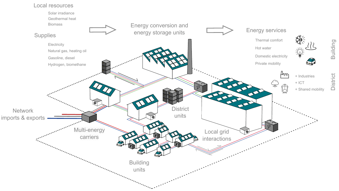
../../_images/district_energy_hub.png — District energy hub: building-scale units are complemented by district-scale conversion and storage units, a shared network interface, and optional district heating/cooling infrastructure.#

Key district additions over the building model:

Decomposition algorithm — tractable MILP for many-building districts
Demand profile pooling — realistic aggregated peaks via stochastic perturbation
District heating/cooling networks — pipe sizing and connection decisions
Local mobility services — multi-modal transport at community scale
Grid reinforcement — transformer and line capacity upgrades
District renovation — envelope decisions integrated in the master problem

Dantzig–Wolfe decomposition#

Principle#

Rather than solving a single monolithic MILP over all buildings, the DWD decomposes the problem into:

A master problem (MP) that selects a convex combination of pre-generated building configurations and optimizes district-level variables (shared infrastructure, network).
Building subproblems (SPs) — one per building — that generate new attractive configurations in response to price signals (dual variables) from the master problem.

This iterative procedure generates a decreasing sequence of upper bounds and an increasing sequence of lower bounds that converge to the optimal district solution.

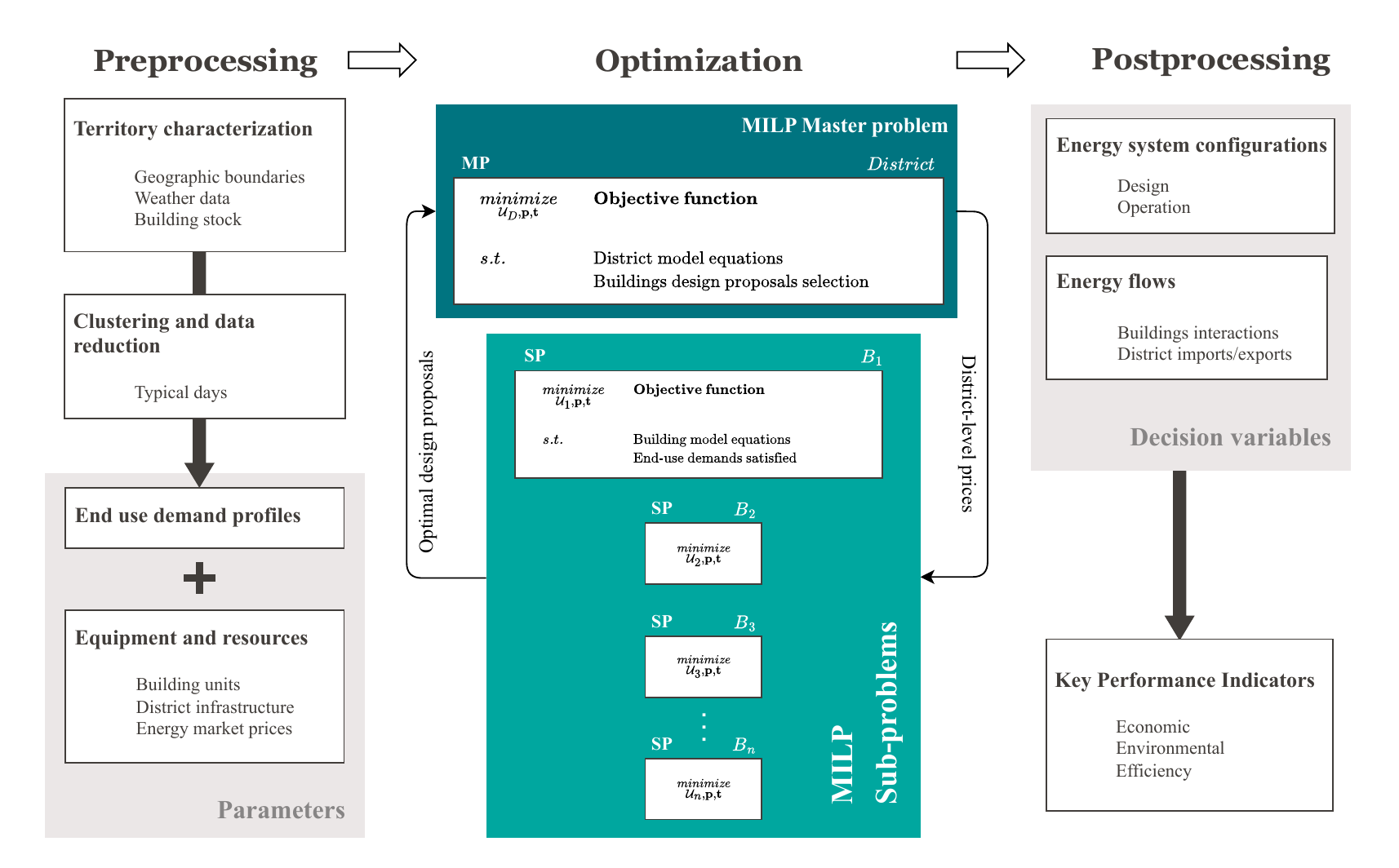
../../_images/decomposition_workflow.png — Dantzig–Wolfe decomposition workflow.#

Master problem#

Configuration selection#

Each building \(b\) is represented as a convex combination of feasible configurations \(f \in \mathbb{F}\) generated by the subproblems:

(1)#\[\sum_{f \in \mathbb{F}} \boldsymbol{\lambda}_{f,b} = 1, \qquad 0 \le \boldsymbol{\lambda}_{f,b} \le 1 \qquad \forall\, b \in \mathbb{B}\]

In the relaxed iterations \(\boldsymbol{\lambda}_{f,b}\) can be fractional; in the final integer solve exactly one configuration per building is selected (\(\boldsymbol{\lambda}_{f,b} \in \{0,1\}\)).

District energy balance#

At every timestep, the aggregate net exchange with the external network equals the sum of all building grid exchanges plus district-unit contributions:

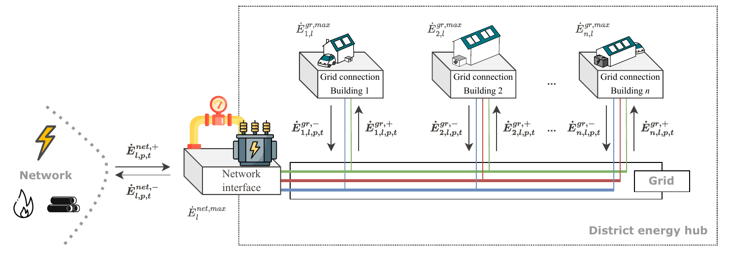
../../_images/DES_balance.png — Energy balance of the district energy system.#

(2)#\[\dot{\boldsymbol{E}}_{l,p,t}^{\text{net},+} - \dot{\boldsymbol{E}}_{l,p,t}^{\text{net},-} = \sum_{f,b} \boldsymbol{\lambda}_{f,b} \bigl(\dot{\boldsymbol{E}}_{f,b,l,p,t}^{\text{gr},+} - \dot{\boldsymbol{E}}_{f,b,l,p,t}^{\text{gr},-}\bigr) + \sum_{u_d \in \mathbb{U_D}} \bigl(\dot{\boldsymbol{E}}_{u_d,l,p,t}^{+} - \dot{\boldsymbol{E}}_{u_d,l,p,t}^{-}\bigr) \qquad \forall\, l,p,t\]

The dual variable \(\boldsymbol{\pi}_{l,p,t}\) associated with this constraint is the internal energy price — the marginal cost of providing one additional unit of carrier \(l\) at timestep \((p,t)\). Network interface capacity is bounded by:

(3)#\[\dot{\boldsymbol{E}}_{l,p,t}^{\text{net},\pm} \le \dot{E}_{l}^{\text{net,max}} \qquad \forall\, l,p,t\]

District cost objective#

OPEX from external network exchanges:

(4)#\[\boldsymbol{C}^{\text{OPEX}} = \sum_{l,p,t} \bigl(c_l^+\,\dot{\boldsymbol{E}}_{l,p,t}^{\text{net},+} - c_l^-\,\dot{\boldsymbol{E}}_{l,p,t}^{\text{net},-}\bigr)\,d_p\,d_t\]

CAPEX for both building configurations and district-scale units:

(5)#\[\boldsymbol{C}^{\text{CAPEX}} = \frac{i(1+i)^n}{(1+i)^n-1}\bigl(\boldsymbol{C}^{\text{inv}} + \boldsymbol{C}^{\text{rep}}\bigr)\]

\[\boldsymbol{C}^{\text{inv}} = \sum_{f,b} \boldsymbol{\lambda}_{f,b}\,C_{f,b}^{\text{inv}} + \sum_{u_d}\bigl(c_{u_d}^1\,\boldsymbol{y}_{u_d} + c_{u_d}^2\,\boldsymbol{f}_{u_d}\bigr)\]

Total district GWP:

(6)#\[\boldsymbol{GWP}^{\text{op}} = \sum_{l,p,t}\bigl(cc^+_{l,p,t}\,\dot{\boldsymbol{E}}^{\text{net},+}_{l,p,t} - cc^-_{l,p,t}\,\dot{\boldsymbol{E}}^{\text{net},-}_{l,p,t}\bigr)\,d_t\,d_p\]

\[\boldsymbol{GWP}^{\text{constr}} = \sum_{f,b} \boldsymbol{\lambda}_{f,b}\,GWP_{f,b}^{\text{constr}} + \sum_{u_d} \frac{1}{n_{u_d}}\bigl(cc_{u_d}^1\,\boldsymbol{y}_{u_d} + cc_{u_d}^2\,\boldsymbol{f}_{u_d}\bigr)\]

Subproblems#

Each building SP is identical to the single-building MILP from 🏠 Building Model, except that the OPEX term uses internal energy prices \(\boldsymbol{\pi}_{l,p,t}\) (fixed dual variables from the latest MP solution) instead of exogenous tariffs:

(7)#\[\boldsymbol{C}_b^{\text{OPEX}} = \sum_{l,p,t} \bigl(\boldsymbol{\pi}_{l,p,t}\,\dot{\boldsymbol{E}}_{b,l,p,t}^{\text{gr},+} - \boldsymbol{\pi}_{l,p,t}\,\dot{\boldsymbol{E}}_{b,l,p,t}^{\text{gr},-}\bigr)\,d_p\,d_t \qquad \forall\, b \in \mathbb{B}\]

The SP objective is:

(8)#\[\min\; \boldsymbol{C}_b^{\text{OPEX}} + \boldsymbol{C}_b^{\text{CAPEX}} - \mu_b\]

A configuration has negative reduced cost (i.e., it improves the MP bound) when the SP objective value is negative. Such configurations are added to the global pool \(\mathbb{F}\) and the MP is re-solved on the enlarged set.

Dual variables#

Three dual variables emerge from the MP and steer the SP searches:

Variable	Constraint	Interpretation
\(\boldsymbol{\pi}_{l,p,t}\)	District energy balance (2)	Internal energy price [CHF/kWh] or marginal GWP [kgCO₂eq/kWh]
\(\boldsymbol{\mu}_b\)	Convexity (1)	Marginal value of integrating building \(b\) into the district
\(\boldsymbol{\beta}\)	MOO \(\epsilon\)-constraint	Local gradient of the Pareto frontier

When the district objective is economic (TOTEX/OPEX), \(\boldsymbol{\pi}\) gives internal prices; when environmental (GWP), it gives marginal carbon impacts.

In multi-objective mode, \(\boldsymbol{\beta}\) is passed to the SPs as an additional weight on the secondary objective, guiding the search toward configurations that are better on the Pareto frontier.

Algorithm workflow#

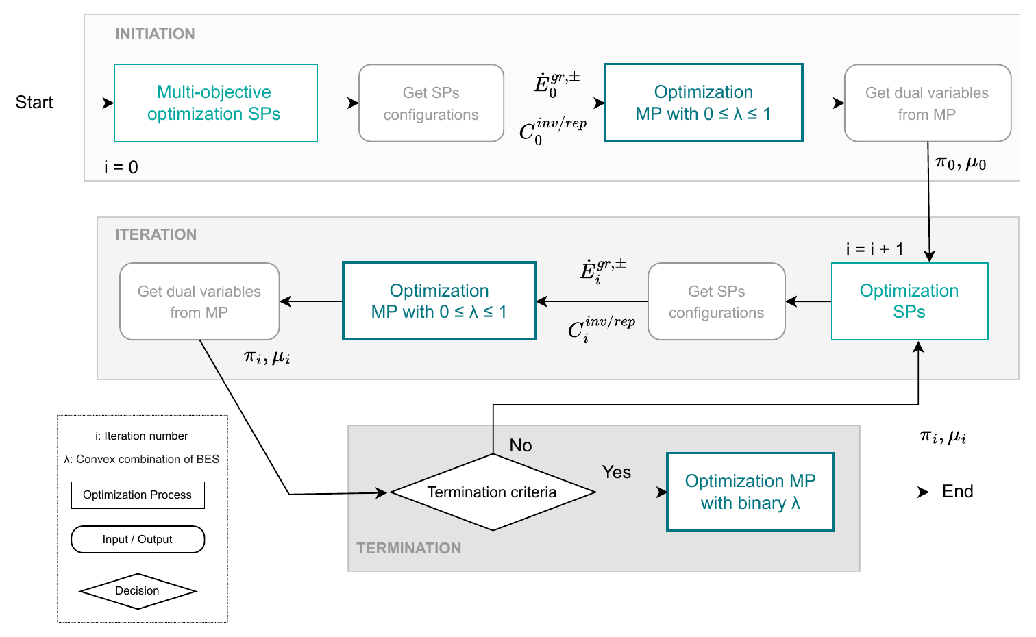
../../_images/decomposition_algorithm.png — Decomposition algorithm flowchart.#

Phase 1 — Initiation:

Solve one compact optimization per building using exogenous energy prices (no district coupling).
Collect the resulting configurations as the initial pool \(\mathbb{F}\).
Solve the first relaxed MP (\(0 \le \boldsymbol{\lambda}_{f,b} \le 1\)) to obtain initial dual variables \(\boldsymbol{\pi}\), \(\boldsymbol{\mu}\) (and \(\boldsymbol{\beta}\) if MOO).

Phase 2 — Iteration:

Pass \(\boldsymbol{\pi}\), \(\boldsymbol{\mu}\) to all SPs as fixed parameters.
Each building SP searches for its configuration with the lowest reduced cost.
If any SP finds a negative reduced-cost configuration, add it to \(\mathbb{F}\).
Re-solve the relaxed MP on the enlarged pool; obtain new dual variables.
Repeat until no SP can find a negative reduced-cost configuration (or until a maximum iteration count is reached).

Phase 3 — Finalization:

Solve a final integer MP with \(\boldsymbol{\lambda}_{f,b} \in \{0,1\}\) to select one configuration per building.
Post-process to compute all district KPIs.

Note

Typical convergence: the gap between the relaxed (lower-bound) and integer (upper-bound) MP objectives is below 0.01% within a few dozen iterations.

The SP solves are independent across buildings and can be parallelized across CPU cores, significantly reducing wall-clock time for large districts.

Demand profile pooling#

Norm-based profiles (SIA 2024) are inherently synchronous across buildings, producing unrealistically large peaks when aggregated. Two independent stochastic perturbations are applied per building to introduce diversity while preserving annual energy demand.

Amplitude factor#

Each building receives an amplitude scaling factor drawn from a normal distribution:

(9)#\[a_b \sim \mathcal{N}(\mu_a, \sigma_a^2) \qquad\Rightarrow\qquad \tilde{e}_{b,p,t} = a_b\,\dot{e}^{0}_{b,p,t}\]

with \(\mu_a \approx 1\) (preserving the norm average) and \(\sigma_a \in [0.1, 0.2]\).

Time-shift factor#

A random hourly lag (advance or delay) is applied:

(10)#\[ts_b \sim \mathcal{N}(\mu_{\text{ts}}, \sigma_{\text{ts}}^2) \qquad\Rightarrow\qquad \dot{e}_{b,p,t} = \tilde{e}_{b,p,t}(1-|ts_b|) + \tilde{e}_{b,p,t\pm1}|ts_b|\]

with \(\mu_{\text{ts}} = 0\) and \(\sigma_{\text{ts}} \approx 1\)–2 h. Linear interpolation between adjacent hours maintains hourly resolution.

Aggregated effect#

The district-level demand is the sum over all buildings:

(11)#\[\dot{e}^{\text{agg}}_{p,t} = \sum_{b \in \mathbb{B}} \dot{e}_{b,p,t}\]

The combined stochastic perturbation reduces aggregated peak power by ~40% and replaces sharp synchronized peaks with smoother, more realistic demand curves. The method applies to all norm-based profiles: electricity, DHW, occupancy, internal gains, ICT, and mobility.

District-scale infrastructure#

District units follow the same black-box formulation as building units (see 🏠 Building Model, Technologies) but are sized and operated at utility scale. Available district technologies include large-scale boilers, geothermal heat pumps, batteries, hydrogen storage, data centers, PTES, rSOC, and methanators.

District heating and cooling networks#

DHC networks allow buildings to exchange heat with centralized sources and sinks.

Temperature levels#

Architecture	Temperature range	Advantages	Drawbacks
High-temperature	> 65 °C	Direct DHW/radiator use, smaller pipes	Higher losses, insulation required
Anergy / low-temperature	~ambient	Minimal losses, compatible with heat pumps	Widespread temperature lifting needed

Two-phase CO₂ loops are also supported (high transfer coefficients, compact piping, isothermal operation).

Deployment cost#

Service pipe diameter is sized from the maximum hourly heat duty:

(12)#\[D_b \ge \left(\frac{4\,\dot{E}^{\text{gr},-}_{b,\text{heat},p,t}}{\pi\,v\,\rho\,\Delta h}\right)^{1/2} \qquad \forall\, b,p,t\]

Total network investment cost:

(13)#\[\boldsymbol{C}^{\text{inv}}_{\text{dhn}} = \sum_{b \in \mathbb{B}} L \bigl(c^{\text{dhn,1}}\,\boldsymbol{y}^{\text{dhn}}_b + c^{\text{dhn,2}}\,D_b\bigr)\]

where the inter-building pipe length is estimated by a geometric surrogate:

(14)#\[L = K \cdot \frac{N-1}{N} \cdot \left(\frac{A^{\text{district}}}{N}\right)^{1/2}\]

with shape factor \(K\), number of buildings \(N\), and total district footprint \(A^{\text{district}}\).

Heat exchanger (HEX) at the building interface#

Each connected building needs a heat exchanger sized to handle peak demand. Its capacity is bounded by the exchanger area \(\boldsymbol{A}^{\text{hex}}_b\):

\[\dot{\boldsymbol{E}}^{\text{hex},-}_{b,\text{heat},p,t} \le \eta^{\text{in}}_b\,U_{\text{hex}}\,\boldsymbol{A}^{\text{hex}}_b\,T^{\text{in}}_{m,b}\]

\[\dot{\boldsymbol{E}}^{\text{hex},+}_{b,\text{heat},p,t} \le \eta^{\text{out}}_b\,U_{\text{hex}}\,\boldsymbol{A}^{\text{hex}}_b\,T^{\text{out}}_{m,b}\]

Temperature feasibility coefficients \(\eta^{\text{in}}_b\), \(\eta^{\text{out}}_b\) (0 or 1) encode whether the DHC supply/return temperatures are compatible with the building’s heat cascade.

Local mobility services#

At district scale, all passenger transport (commuting, leisure, errands) is aggregated on a dedicated Mobility energy layer. Multiple modes are available: EVs, ICE vehicles, bicycles, e-bikes, and public transport.

Demand and distance classes#

The daily mobility demand is segmented by distance class \(d \in \mathbb{D}\) (e.g., short, medium, long trips):

(15)#\[D^{\text{mob}}_{d,p,t} = \phi^{\text{dem}}_{\tau(p),d,t}\,D^{\text{day}}_d\,N^{\text{pop}} \qquad \forall\, d,p,t\]

where \(\phi^{\text{dem}}_{\tau,d,t}\) is a normalized hourly profile (weekday/weekend), \(D^{\text{day}}_d\) [km/person/day] the average daily distance for class \(d\), and \(N^{\text{pop}}\) the district population.

EV fleet model#

The EV battery energy is split between vehicles plugged in at the district (\(\boldsymbol{E}^{\text{ev,on}}_{p,t}\)) and those away (\(\boldsymbol{E}^{\text{ev,off}}_{p,t}\)):

(19)#\[\boldsymbol{E}^{\text{ev}}_{p,t} = \boldsymbol{E}^{\text{ev,on}}_{p,t} + \boldsymbol{E}^{\text{ev,off}}_{p,t}\]

The plugged-in energy evolves as:

(20)#\[\boldsymbol{E}^{\text{ev,on}}_{p,t} = \sigma_{\text{EV}}\,\boldsymbol{E}^{\text{ev}}_{p,t-1}\,\alpha_{p,t} - \boldsymbol{E}^{\text{ev,displ}}_{p,t} + \eta^-\,\boldsymbol{E}^{\text{ev,+}}_{p,t} - \frac{1}{\eta^+}\,\boldsymbol{E}^{\text{ev,-}}_{p,t}\]

where \(\alpha_{p,t}\) is the plug-on fraction (vehicles available for charging), \(\boldsymbol{E}^{\text{ev,displ}}_{p,t}\) is driving energy, and \(\eta^{\pm}\) are charge/discharge efficiencies.

SoC bounds are enforced separately for plugged-in and plugged-out vehicles, and cyclic constraints close the SoC over each typical period.

Unidirectional (smart charging): \(\boldsymbol{E}^{\text{ev,-}}_{p,t} = 0\) — no vehicle-to-grid.
Bidirectional (V2G/V2D): \(\boldsymbol{E}^{\text{ev,-}}_{p,t}\) is a decision variable, enabling EVs to inject electricity back into the district.

Public transport and active modes#

Public transport appears as an external supply on the Mobility layer (import at associated cost and GWP). Conventional bicycles have zero energy consumption. E-bikes consume a small amount of electricity proportional to km ridden.

Grid reinforcement#

Two types of reinforcement are modeled: the network interface (e.g., HV/MV transformer) and individual building-to-grid lines.

Network interface#

The network capacity \(\boldsymbol{f}^{\text{net}}_l\) is chosen from a discrete catalogue \(\mathbb{G}^{\text{net}}_l\) of standard transformer ratings, respecting the existing capacity \(f^{\text{ex,net}}_l\):

(21)#\[\boldsymbol{f}^{\text{net}}_l \ge f^{\text{ex,net}}_l, \quad \boldsymbol{f}^{\text{net}}_l \in \mathbb{G}^{\text{net}}_l, \quad \dot{\boldsymbol{E}}^{\text{net},\pm}_{l,p,t} \le \boldsymbol{f}^{\text{net}}_l\]

Investment cost includes a fixed activation term and a proportional capacity term:

(22)#\[\boldsymbol{C}^{\text{inv,net}}_l = c^{\text{net,1}}_l\,\boldsymbol{y}^{\text{net}}_l + c^{\text{net,2}}_l \bigl(\boldsymbol{f}^{\text{net}}_l - f^{\text{ex,net}}_l(1 - \boldsymbol{y}^{\text{net}}_l)\bigr)\]

Building-to-grid lines#

Each building-layer pair has its own line capacity, similarly selected from a discrete catalogue:

(23)#\[\boldsymbol{f}^{\text{gr}}_{b,l} \ge f^{\text{ex,gr}}_{b,l}, \quad \boldsymbol{f}^{\text{gr}}_{b,l} \in \mathbb{G}^{\text{gr}}_l, \quad \dot{\boldsymbol{E}}^{\text{gr},\pm}_{b,l,p,t} \le \boldsymbol{f}^{\text{gr}}_{b,l} \qquad \forall\, b,l,p,t\]

Renovation at district scale#

At district scale the master problem selects one configuration per building from the pool \(\mathbb{F}_b\) that now includes renovation options (see 🏠 Building Model). Each configuration carries:

Effective envelope coefficient \(U_{f,b}\)
Renovation cost \(C^{\text{ren}}_{f,b}\) and embodied GWP \(\mathrm{GWP}^{\text{ren}}_{f,b}\)
Operational performance from the SP

Aggregate renovation cost and GWP are obtained by weighting:

(24)#\[\boldsymbol{C}^{\text{ren}}_b = \sum_{f} C^{\text{ren}}_{f,b}\,\boldsymbol{\lambda}_{f,b} \qquad \boldsymbol{\mathrm{GWP}}^{\text{ren}}_b = \sum_{f} \mathrm{GWP}^{\text{ren}}_{f,b}\,\boldsymbol{\lambda}_{f,b} \qquad \forall\, b \in \mathbb{B}\]

A minimum renovation share constraint enforces that at least a fraction \(\gamma^{\text{ren}}\) of total district floor area is renovated: